Training-3

Scalable Approaches for Large-Scale Genetic Association Analyses

Summary: Genome-wide association studies (GWAS) are crucial for identifying genetic variants associated with complex traits and diseases, providing insights into biology and potential therapeutic targets. However, GWAS rely on large sample sizes, creating a demand for highly scalable software to handle such massive datasets efficiently. In this training, we will explore three tools designed to perform GWAS on large-scale datasets (e.g., UK Biobank with 500k individuals and millions of variants to be tested): REGENIE [1], fastGWA/fastGWA-GLMM [2,3,4], and CMA [5]. The session will include a basic explanation of the fundamental principles underlying the software and practical demonstrations of how to run these tools on publicly available datasets. For curious readers, some mathematical details of these tools are also provided in this material, although they are not intended to be covered in depth during the training.

Objective: This training aims to provide an applied session on running large-scale GWAS using REGENIE, fastGWA/fastGWA-GLMM, and CMA. While we will briefly touch on the underlying theory, the main emphasis will be on hands-on demonstrations with publicly available datasets.

Brief Overview of GWAS
Installing the Software and Dataset
Introduction to fastGWA and fastGWA-GLMM
Running GWAS with fastGWA and fastGWA-GLMM
☕ Coffee break (15 mins)
Introduction to REGENIE
Running GWAS with REGENIE
Introduction to CMA
Running GWAS with CMA
(Optional) Running Meta-Analysis with CMA
💬 Questions / Comments / Feedback
References

⬤ Coding Session
⬤ Concepts & Theory

Brief Overview of GWAS

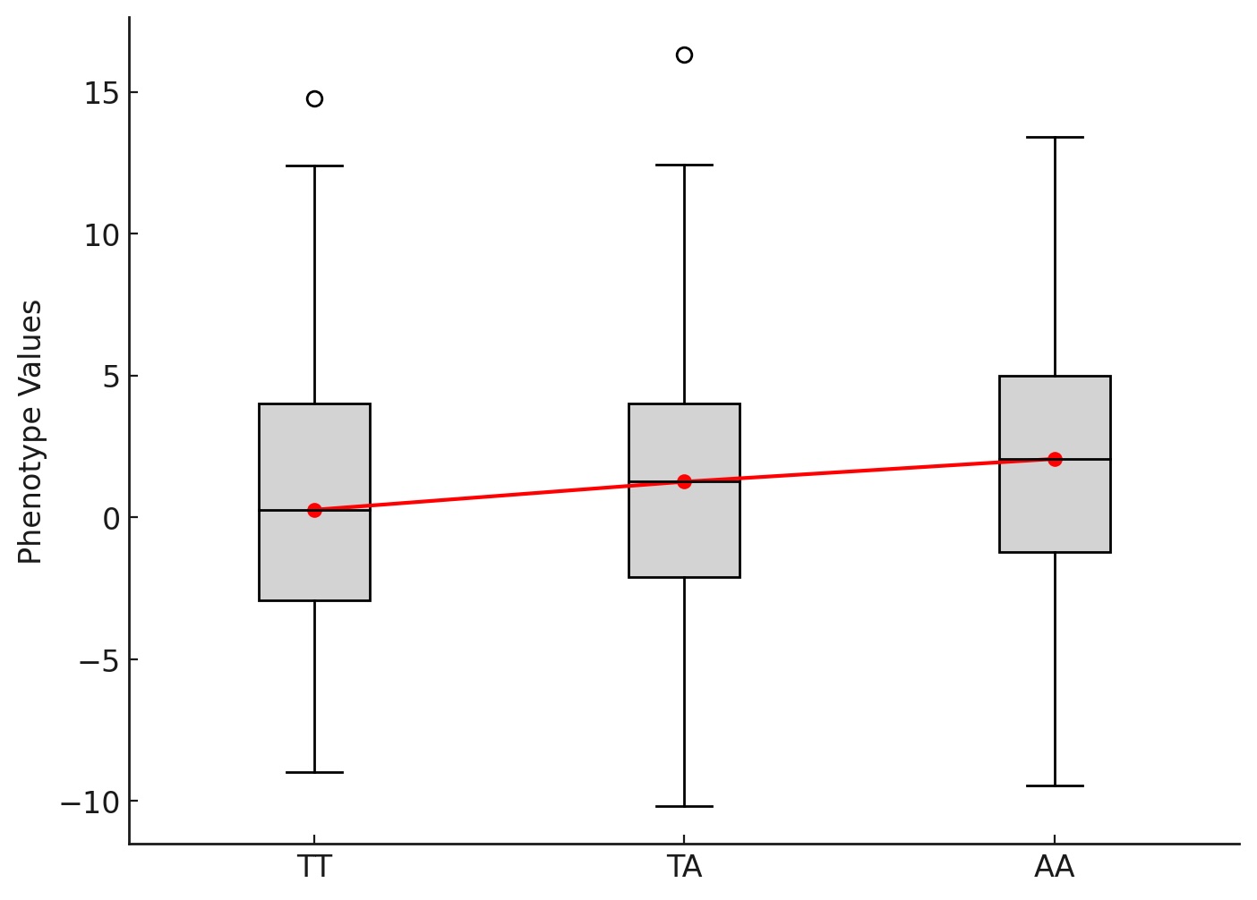
A genome-wide association study (GWAS) is a research approach used to identify genetic variants associated with specific traits or diseases by scanning the genomes of many individuals. In GWAS, researchers compare the frequency of single-nucleotide polymorphisms (SNPs) across the entire genome between individuals with different trait values, such as cases versus controls for a disease (binary traits) or variations in a continuous measurement like height or blood pressure (quantitative traits). This method can reveal genetic risk factors without prior knowledge of candidate genes, making it especially powerful for studying complex traits influenced by many genes and environmental factors. Insights from GWAS contribute to understanding biological pathways, improving disease risk prediction, and guiding precision medicine efforts.

Simple Linear Regression in GWAS:

\[ y = g \cdot \beta_g + \epsilon \]

Where:

$y$: Trait or phenotype values for individuals
$g$: Genotype coding for the variant (e.g., # of A alleles: 0, 1, or 2)
$\beta_g$: Estimated effect size of the genotype on the phenotype
$\epsilon$: Random error term

Confounders in GWAS:

Population structure
Related individuals
Linkage disequilibrium (LD)

Check the YouTube video for more information: Watch on YouTube

Linear Mixed Models (LMMs) in GWAS

\[ y = X\beta + g_j \beta_j + u + \epsilon \]

Where:

$y$: Phenotype vector ($n \times 1$) for all individuals
$X\beta$: Fixed effects for non-genetic covariates (e.g., age, sex, principal components)
$g_j \beta_j$: Fixed effect of the $j$-th genetic variant being tested
$u$: Polygenic random effect, $u \sim N(0, \sigma_g^2 K)$
- $K$: Genetic relationship matrix (GRM), often stored in sparse form for efficiency (it can be computed from genotype data)
- $\sigma_g^2$: Genetic variance component
$\epsilon$: Residual error, $\epsilon \sim N(0, \sigma_e^2 \mathbf{I})$

Solving LMMs in GWAS

The generalised least squares estimate $\widehat{\beta}_j$ of the effect size of $g_j$ is obtained as:

\[ \widehat{\beta}_j = \frac{g_j^{T} \mathbf{V}^{-1} y}{g_j^{T} \mathbf{V}^{-1} g_j} \]

where $\mathbf{V}$ is the variance–covariance matrix of the phenotype, incorporating both polygenic and residual variance components:
\[ \mathbf{V} = K\cdot\sigma_g^2+\mathbf{I}\cdot\sigma_e^2 \]

The corresponding variance of $\widehat{\beta}_j$ is:

\[ \mathrm{Var}(\widehat{\beta}_j) = (g_j^{T} \mathbf{V}^{-1} g_j)^{-1} \] The only unknowns in this solution are the variance components $\sigma^2_g$ and $\sigma^2_e$, which are estimated using efficient restricted maximum likelihood (REML) methods.

Hypothesis Testing in GWAS (LMMs)

In GWAS, statistical hypothesis testing is performed to determine whether a given genetic variant is associated with a trait of interest.
For each variant, we assess the following competing hypotheses:

\[ \begin{aligned} H_0: & \quad \beta_j = 0 & \text{(no association between variant $ g_j $ and phenotype $ y $)} \\ H_1: & \quad \beta_j \neq 0 & \text{(variant $ g_j $ is associated with $ y $)} \end{aligned} \]

Under the null hypothesis $H_0$, the squared Wald statistic is given by: \[ T_j^2 = \frac{\widehat{\beta}_j^2}{\mathrm{Var}(\widehat{\beta}_j)} \;\sim\; \chi^2_1 \] where $\widehat{\beta}_j$ is the estimated effect size and $\mathrm{Var}(\widehat{\beta}_j)$ its variance.

The statistical significance for variant $j$ is assessed by: \[ p_j = 1 - F_{\chi^2_1}(T_j^2) \] where $F_{\chi^2_1}(\cdot)$ is the cumulative distribution function of the chi-square distribution with 1 degree of freedom.

Evidence of Association in GWAS LMMs

A small $p$-value suggests rejecting $H_0$ in favour of $H_1$, meaning the variant is more likely to be associated with the trait. This naturally leads to the question: how small must the $p$-value be to consider the evidence convincing?

In GWAS, where millions of variants are tested, a stringent genome wide significance threshold is applied, often $p < 5 \times 10^{-8}$. This threshold approximates a Bonferroni correction for about one million effectively independent tests and addresses the challenge known as the multiple testing problem in GWAS.

Why use a stringent threshold in GWAS?
In GWAS, millions of variants ($M$) are tested across the genome. The expected number of false positives is approximately $M \times \alpha$, where $\alpha$ is the chosen significance level.
Without adjustment, using a conventional $\alpha = 0.05$ would yield thousands of false positives purely by chance.
This motivates the adoption of a much smaller threshold, such as $5 \times 10^{-8}$, to keep the average number of false positives at a reasonable level.

Key idea in LMMs:
Linear mixed models account for both fixed and random effects, helping to control for confounders while efficiently testing the association between each genetic variant and the phenotype.

Note on LOCO (Leave-One-Chromosome-Out):
GWAS methods use a LOCO scheme when generating polygenic predictions or fitting random effects.
In LOCO, the genetic relationship matrix (or polygenic score) is calculated excluding the chromosome currently being tested.
This prevents “proximal contamination” [6].

GWAS Requires Large Sample Sizes

Genome-wide association studies typically test millions of genetic variants across the genome. Because each variant often explains only a very small fraction of the variation in a trait, detecting true associations with sufficient statistical power requires large numbers of participants. Larger sample sizes reduce random noise, improve the precision of effect size estimates, and help identify variants with small effects that would be missed in smaller datasets. This scale of data creates a strong need for highly efficient and scalable computational tools that can process and analyse results within a reasonable time frame and with optimal computational resources.

Installing the Software and Dataset

This training course covers scalable GWAS tools REGENIE, fastGWA/fastGWA-GLMM, and CMA, all using the same prepared dataset and a shared set of software dependencies. Follow the steps below to set up your environment, install the required software, and download the dataset for use throughout the course.

Clone the CMA Repository (includes setup instructions for the software and dataset)
```
git clone https://git.ecdf.ed.ac.uk/cma/snake-cma.git
```

Install dependencies — choose one of the following:

Using Conda (recommended)

conda env create -f snake-cma/environment.yml
conda activate snake-cma

Using Pip

pip install -r snake-cma/requirements.txt

Download the example dataset and software binaries
The provided scripts will download static versions of PLINK, REGENIE, and GCTA (contains fastGWA and fastGWA-GLMM), and generate the HapMap3-based dataset that will be used in all hands-on sessions.
```
chmod +x ./snake-cma/examples/download_software.sh ./snake-cma/examples/generate_dataset.sh

bash ./snake-cma/examples/download_software.sh
bash ./snake-cma/examples/generate_dataset.sh
```
This will create:
- ./snake-cma/examples/software/ — Contains required software: REGENIE, fastGWA/fastGWA-GLMM, and CMA
- ./snake-cma/examples/data/ — Contains required dataset used in exercises

Before starting any tutorial, ensure your snake-cma environment is active (if not already):

conda activate snake-cma

Next, save the current working directory (location of the cloned snake-cma repository) into a variable. This will be reused throughout the tutorial.

dir_user=$(pwd)

At this point, you can quickly check that the example dataset has been generated correctly by listing its contents:

ls -lh ${dir_user}/snake-cma/examples/data

The data folder should contain the following files:

File	Content
`binary_trait.phen`	Phenotype file for a binary trait (BT).
`continuous_trait.phen`	Phenotype file for a quantitative trait (QT).
`HAPMAP3.covars.cov`	Covariate file for REGENIE.
`HAPMAP3.covars.qcovar`	Covariate file for fastGWA/fastGWA-GLMM (Quantitative)
`HAPMAP3.covars.bcovar`	Covariate file for fastGWA/fastGWA-GLMM (Discrete)
`HAPMAP3.qc.genotype.{bed,bim,fam}`	Genotype files in PLINK binary format (`.bed`, `.bim`, `.fam`).

Introduction to fastGWA and fastGWA-GLMM

fastGWA is an efficient mixed linear model (MLM) approach implemented in the GCTA software for genome-wide association studies that can handle large cohorts while accounting for population structure and relatedness. It achieves speed by using a sparse genetic relationship matrix (GRM), which stores only relationships above a certain relatedness threshold, dramatically reducing memory and computational costs compared to a full GRM. This makes fastGWA well suited for quantitative traits in biobank-scale datasets.

fastGWA-GLMM is an extension of fastGWA designed for binary traits, using a generalized linear mixed model to correctly model case–control outcomes while still leveraging the sparse GRM for computational efficiency. By fitting the model on the observed binary phenotype and using approximate inference, fastGWA-GLMM can scale to millions of variants and hundreds of thousands of individuals while maintaining control over confounding from relatedness and population stratification.

Linear Mixed Model for Quantitative Traits

For a given genetic variant $j$:

\[ y = X\beta + g_j \alpha_j + u + \epsilon \]

Where:

$y$: Phenotype vector ($n \times 1$)
$X$: Covariate matrix (e.g., age, sex, principal components)
$\beta$: Fixed effect coefficients for covariates
$g_j$: Genotype vector for variant $j$ (0, 1, 2 dosage)
$\alpha_j$: Effect size of variant $j$
$u$: Polygenic random effect, $u \sim N(0, \sigma_g^2 K)$
- $K$: Genetic relationship matrix (GRM), often sparse for efficiency
$\epsilon$: Residual error, $\epsilon \sim N(0, \sigma_e^2 \mathbf{I})$

The null hypothesis $H_0: \alpha_j = 0$ is tested for each variant.

Generalized Linear Mixed Model for Binary Traits

For binary phenotypes ($y_i \in \{0,1\}$), a logistic link is used:

\[ \text{logit}\left[ P(y = 1) \right] = X \beta + g_{j} \alpha_j + u \]

Where:

$\text{logit}(p) = \log \left( \frac{p}{1-p} \right)$
$u \sim N(0, \sigma_g^2 K)$ models genome-wide background effects
The residual variance is absorbed in the logistic model framework

Computational Note

Both fastGWA and fastGWA-GLMM models estimate $\sigma_g^2$ and $\sigma_e^2$ once under the null and reuse them across variants.
Using a sparse GRM drastically reduces memory and computation.

Running GWAS with fastGWA and fastGWA-GLMM

We will follow the instructions from the GCTA website to perform GWAS using fastGWA and fastGWA-GLMM.

EXERCISE 1: Running fastGWA Interactively (Quantitative Trait)

dir_data=${dir_user}/snake-cma/examples/data
dir_cma=${dir_user}/snake-cma/examples/cma-tests

mkdir -p ${dir_cma}

geno=${dir_data}/HAPMAP3.qc.genotype
pheno=${dir_data}/continuous_trait.phen
covars=${dir_data}/HAPMAP3.covars.cov
output=${dir_cma}/ex1-gcta-qt
grm=${dir_data}/HAPMAP3.qc.genotype.grm_matrix

gcta=${dir_user}/snake-cma/examples/software/gcta64/gcta-1.94.4-linux-kernel-3-x86_64/gcta64

echo Starting..

# Build sparse GRM only if it doesn't exist
if [ ! -f "${grm}.grm.sp" ]; then
  ${gcta} --bfile ${geno} \
      --make-grm \
      --sparse-cutoff 0.05 \
      --out ${grm}
fi

${gcta} --bfile ${geno} \
    --grm-sparse ${grm} \
    --fastGWA-mlm \
    --pheno ${pheno} \
    --qcovar ${covars} \
    --out ${output}

echo Done..

Once the analysis is complete, you can inspect the output summary statistics generated by fastGWA. The results file contains genome information such as CHR (chromosome), SNP (variant identifier), and POS (base-pair position), along with association results such as BETA (effect size estimate), SE (standard error of the effect size), and P (p-value for association). These columns allow you to interpret the strength and direction of association between each variant and the phenotype.

EXERCISE 2: Perform GWAS with fastGWA interactively using both –qcovar and –covar options

Goal: Demonstrate how fastGWA automatically transforms discrete covariates into dummy variables and merges quantitative and discrete covariates into a single combined covariate file.

Hint

Use the –qcovar option for continuous (quantitative) covariates and the –covar option for discrete covariates in fastGWA. You need to use HAPMAP3.covars.qcovar and HAPMAP3.covars.bcovar respectively.

Show solution

dir_data=${dir_user}/snake-cma/examples/data
dir_cma=${dir_user}/snake-cma/examples/cma-tests

mkdir -p ${dir_cma}

geno=${dir_data}/HAPMAP3.qc.genotype
pheno=${dir_data}/continuous_trait.phen
qcovars=${dir_data}/HAPMAP3.covars.qcovar
bcovars=${dir_data}/HAPMAP3.covars.bcovar
output=${dir_cma}/ex2-gcta-qt
grm=${dir_data}/HAPMAP3.qc.genotype.grm_matrix

gcta=${dir_user}/snake-cma/examples/software/gcta64/gcta-1.94.4-linux-kernel-3-x86_64/gcta64

echo Starting..

# Build sparse GRM only if it doesn't exist
if [ ! -f "${grm}.grm.sp" ]; then
  ${gcta} --bfile ${geno} \
      --make-grm \
      --sparse-cutoff 0.05 \
      --out ${grm}
fi

${gcta} --bfile ${geno} \
    --grm-sparse ${grm} \
    --fastGWA-mlm \
    --pheno ${pheno} \
    --qcovar ${qcovars} \
    --covar ${bcovars} \
    --out ${output}

echo Done..

EXERCISE 3: Run GWAS with fastGWA via a Bash script

Goal: Write and run a small Bash script that builds a sparse GRM (if missing) and runs fastGWA for a quantitative trait. Make sure to change the output variable to a unique name before running.

Show solution

Create the script file:
```
nano ex3.sh
```

Paste the solution below, then save and close:

#!/bin/bash
set -euo pipefail

dir_user="${1:?ERROR: provide repo root as first argument}"
dir_data="${dir_user}/snake-cma/examples/data"
dir_cma="${dir_user}/snake-cma/examples/cma-tests"

mkdir -p "${dir_cma}"

geno="${dir_data}/HAPMAP3.qc.genotype"
pheno="${dir_data}/continuous_trait.phen"
covars="${dir_data}/HAPMAP3.covars.cov"
output="${dir_cma}/ex3-gcta-qt"
grm="${dir_data}/HAPMAP3.qc.genotype.grm_matrix"

gcta="${dir_user}/snake-cma/examples/software/gcta64/gcta-1.94.4-linux-kernel-3-x86_64/gcta64"

echo "Starting.."

# Build sparse GRM only if it doesn't exist
if [ ! -f "${grm}.grm.sp" ]; then
  "${gcta}" \
    --bfile "${geno}" \
    --make-grm \
    --sparse-cutoff 0.05 \
    --out "${grm}"
fi

"${gcta}" \
  --bfile "${geno}" \
  --grm-sparse "${grm}" \
  --fastGWA-mlm \
  --pheno "${pheno}" \
  --qcovar "${covars}" \
  --out "${output}"

echo "Done.."

Run the script (pass the repository root you saved earlier as dir_user):
```
bash ex3.sh "${dir_user}"
```

EXERCISE 4 (Optional): Run GWAS with fastGWA using an HPC job script on your cluster

Goal: Write and run a small job script for your local HPC cluster that builds a sparse GRM (if missing) and runs fastGWA for a quantitative trait. Make sure to change the output variable to a unique name before running.

Show solution

A solution for Eddie (the University of Edinburgh HPC cluster) will be provided during the in-person training.

EXERCISE 5: Running fastGWA-GLMM Interactively (Binary Trait)

dir_data=${dir_user}/snake-cma/examples/data
dir_cma=${dir_user}/snake-cma/examples/cma-tests

mkdir -p ${dir_cma}

geno=${dir_data}/HAPMAP3.qc.genotype
pheno=${dir_data}/binary_trait.phen
covars=${dir_data}/HAPMAP3.covars.cov
output=${dir_cma}/ex5-gcta-bt
grm=${dir_data}/HAPMAP3.qc.genotype.grm_matrix

gcta=${dir_user}/snake-cma/examples/software/gcta64/gcta-1.94.4-linux-kernel-3-x86_64/gcta64

echo Starting..

# Build sparse GRM only if it doesn't exist
if [ ! -f "${grm}.grm.sp" ]; then
  ${gcta} --bfile ${geno} \
      --make-grm \
      --sparse-cutoff 0.05 \
      --out ${grm}
fi

${gcta} --bfile ${geno} \
    --grm-sparse ${grm} \
    --fastGWA-mlm-binary \
    --pheno ${pheno} \
    --qcovar ${covars} \
    --joint-covar \
    --out ${output}

echo Done..

EXERCISE 6: Run GWAS with fastGWA-GLMM via a Bash script

Goal: Write and run a small Bash script that builds a sparse GRM (if missing) and runs fastGWA-GLMM for a binary trait. Make sure to change the output variable to a unique name before running.

Show solution

Create the script file:
```
nano ex6.sh
```

Paste the solution below, then save and close:

#!/bin/bash
set -euo pipefail

dir_user="${1:?ERROR: provide repo root as first argument}"
dir_data="${dir_user}/snake-cma/examples/data"
dir_cma="${dir_user}/snake-cma/examples/cma-tests"

mkdir -p "${dir_cma}"

geno="${dir_data}/HAPMAP3.qc.genotype"
pheno="${dir_data}/binary_trait.phen"
covars="${dir_data}/HAPMAP3.covars.cov"
output="${dir_cma}/ex6-gcta-bt"
grm="${dir_data}/HAPMAP3.qc.genotype.grm_matrix"

gcta="${dir_user}/snake-cma/examples/software/gcta64/gcta-1.94.4-linux-kernel-3-x86_64/gcta64"

echo "Starting.."

# Build sparse GRM only if it doesn't exist
if [ ! -f "${grm}.grm.sp" ]; then
  "${gcta}" \
    --bfile "${geno}" \
    --make-grm \
    --sparse-cutoff 0.05 \
    --out "${grm}"
fi

"${gcta}" \
  --bfile "${geno}" \
  --grm-sparse "${grm}" \
  --fastGWA-mlm-binary \
  --joint-covar \
  --pheno "${pheno}" \
  --qcovar "${covars}" \
  --out "${output}"

echo "Done.."

Run the script (pass the repository root you saved earlier as dir_user):
```
bash ex6.sh "${dir_user}"
```

EXERCISE 7: Run GWAS with fastGWA-GLMM via a Bash script using only quantitative covariates

Goal: Assess how results differ when including only quantitative covariates compared to using the full set of covariates.

Show solution

Create the script file:
```
nano ex7.sh
```

Paste the solution below, then save and close:

#!/bin/bash
set -euo pipefail

dir_user="${1:?ERROR: provide repo root as first argument}"
dir_data="${dir_user}/snake-cma/examples/data"
dir_cma="${dir_user}/snake-cma/examples/cma-tests"

mkdir -p "${dir_cma}"

geno="${dir_data}/HAPMAP3.qc.genotype"
pheno="${dir_data}/binary_trait.phen"
covars="${dir_data}/HAPMAP3.covars.qcovar"
output="${dir_cma}/ex7-gcta-bt"
grm="${dir_data}/HAPMAP3.qc.genotype.grm_matrix"

gcta="${dir_user}/snake-cma/examples/software/gcta64/gcta-1.94.4-linux-kernel-3-x86_64/gcta64"

echo "Starting.."

# Build sparse GRM only if it doesn't exist
if [ ! -f "${grm}.grm.sp" ]; then
  "${gcta}" \
    --bfile "${geno}" \
    --make-grm \
    --sparse-cutoff 0.05 \
    --out "${grm}"
fi

"${gcta}" \
  --bfile "${geno}" \
  --grm-sparse "${grm}" \
  --fastGWA-mlm-binary \
  --joint-covar \
  --pheno "${pheno}" \
  --qcovar "${covars}" \
  --out "${output}"

echo "Done.."

Run the script (pass the repository root you saved earlier as dir_user):
```
bash ex7.sh "${dir_user}"
```

EXERCISE 8 (Optional): Run GWAS with fastGWA using an HPC job script on your cluster

Goal: write and run a small job script for your local HPC cluster that builds a sparse GRM (if missing) and runs fastGWA-GLMM for a quantitative trait. Make sure to change the output variable to a unique name before running.

Show solution

A solution for Eddie (the University of Edinburgh HPC cluster) will be provided during the in-person training.

EXERCISE 9: Run GWAS with Multiple Phenotypes using fastGWA or fastGWA-GLMM

Goal: fastGWA and fastGWA-GLMM do not support analysing multiple phenotypes in a single run. This exercise shows how to run one phenotype at a time using the –mpheno option.

The example below demonstrates how to run GWAS for the second trait (Y2) when the phenotype file contains two traits, Y1 and Y2.

dir_data="${dir_user}/snake-cma/examples/data"
dir_cma="${dir_user}/snake-cma/examples/cma-tests"

mkdir -p "${dir_cma}"

geno="${dir_data}/HAPMAP3.qc.genotype"
pheno="${dir_data}/binary_trait.phen"
covars="${dir_data}/HAPMAP3.covars.qcovar"
output="${dir_cma}/ex9a-gcta-bt"
grm="${dir_data}/HAPMAP3.qc.genotype.grm_matrix"

gcta="${dir_user}/snake-cma/examples/software/gcta64/gcta-1.94.4-linux-kernel-3-x86_64/gcta64"

# Create another Phenotype file with two trait values (Y1 and Y2)
# We will be using only Y2!

pheno_v2="${dir_data}/binary_trait.v2.phen"
awk 'BEGIN{OFS=" "} NR==1{print $0,"Y2"; next} {L[NR]=$0; Y[++n]=$3} \
     END{srand(); for(i=1;i<=n;i++){j=int(1+rand()*n); t=Y[i]; Y[i]=Y[j]; Y[j]=t} \
     for(i=2;i<=n+1;i++){split(L[i],a,/ +/); print a[1],a[2],a[3],Y[i-1]}}' "${pheno}" > "${pheno_v2}"

echo "Starting.."

# Build sparse GRM only if it doesn't exist
if [ ! -f "${grm}.grm.sp" ]; then
  "${gcta}" \
    --bfile "${geno}" \
    --make-grm \
    --sparse-cutoff 0.05 \
    --out "${grm}"
fi

"${gcta}" \
  --bfile "${geno}" \
  --grm-sparse "${grm}" \
  --fastGWA-mlm-binary \
  --joint-covar \
  --pheno "${pheno_v2}" \
  --mpheno 2 \
  --qcovar "${covars}" \
  --out "${output}"

echo "Done.."

You can also loop over the two traits and run fastGWA or fastGWA-GLMM in a single script, executing two GWAS analyses back to back.

dir_data="${dir_user}/snake-cma/examples/data"
dir_cma="${dir_user}/snake-cma/examples/cma-tests"

mkdir -p "${dir_cma}"

geno="${dir_data}/HAPMAP3.qc.genotype"
pheno="${dir_data}/binary_trait.phen"
covars="${dir_data}/HAPMAP3.covars.qcovar"
output="${dir_cma}/ex9b-gcta-bt"
grm="${dir_data}/HAPMAP3.qc.genotype.grm_matrix"

gcta="${dir_user}/snake-cma/examples/software/gcta64/gcta-1.94.4-linux-kernel-3-x86_64/gcta64"

pheno_v3="${dir_data}/binary_trait.v3.phen"
awk 'BEGIN{OFS=" "} NR==1{print $0,"Y2"; next} {L[NR]=$0; Y[++n]=$3} \
     END{srand(); for(i=1;i<=n;i++){j=int(1+rand()*n); t=Y[i]; Y[i]=Y[j]; Y[j]=t} \
     for(i=2;i<=n+1;i++){split(L[i],a,/ +/); print a[1],a[2],a[3],Y[i-1]}}' "${pheno}" > "${pheno_v3}"

echo "Starting.."

# Build sparse GRM only if it doesn't exist
if [ ! -f "${grm}.grm.sp" ]; then
  "${gcta}" \
    --bfile "${geno}" \
    --make-grm \
    --sparse-cutoff 0.05 \
    --out "${grm}"
fi

for m in 1 2; do
  out=${output}".trait_${m}"
  echo "Running GWAS for phenotype column ${m}..."
  "${gcta}" \
    --bfile "${geno}" \
    --grm-sparse "${grm}" \
    --fastGWA-mlm-binary \
    --joint-covar \
    --pheno "${pheno_v3}" \
    --mpheno ${m} \
    --qcovar "${qcovars}" \
    --out "${out}"
done

echo "Done.."

Note that in GCTA, the default phenotype index is –mpheno 1. This means that if no –mpheno option is specified, GCTA (fastGWA/fastGWA-GLMM) will run GWAS using the first phenotype in the file.

EXERCISE 10 (Optional): Split GRM Calculation

Goal: Practice splitting GRM computation into multiple parts, running them in parallel, and merging them before creating a sparse GRM.

Show solution

# (Optional) Build GRM in parts, then merge

# Example: split GRM into two parts (these can be run in parallel)
${gcta} --bfile ${geno} --make-grm-part 2 1 --thread-num 8 --out ${output}_grm_partial
${gcta} --bfile ${geno} --make-grm-part 2 2 --thread-num 8 --out ${output}_grm_partial

# Merge GRM parts
cat ${output}_grm_partial.part_2_*.grm.id    > ${output}_grm_partial_merged.grm.id
cat ${output}_grm_partial.part_2_*.grm.bin   > ${output}_grm_partial_merged.grm.bin
cat ${output}_grm_partial.part_2_*.grm.N.bin > ${output}_grm_partial_merged.grm.N.bin

# Create a sparse GRM
${gcta} --grm ${output}_grm_partial_merged --make-bK-sparse 0.05 --out ${output}_grm_partial_merged.sparse

☕ Coffee break: We will take a 15-minute break here before continuing with the tutorial.

Introduction to REGENIE

REGENIE is a whole-genome regression method optimised for performing GWAS efficiently in large datasets. It employs a two-step approach: In Step 1, a two-level ridge regression model is fit to a subset of genetic variants to capture polygenic effects. This step generates leave-one-chromosome-out (LOCO) predictions of phenotypes. In Step 2, individual genetic variants are tested for association with the trait, adjusting for the LOCO predictions to account for polygenic effects and potential confounders. The key computational innovation of REGENIE lies in Step 1, where the genotype matrix is divided into large blocks. Each block undergoes first-level ridge regression to generate intermediate predictors, which are then combined in a second-level ridge regression to produce LOCO predictions for the trait. This block-wise parallelisation significantly reduces the computational burden, enabling the method to scale to datasets with hundreds of thousands of samples while preserving accuracy. REGENIE’s efficiency makes it particularly well-suited for large-scale biobank studies, where high computational demands are common.

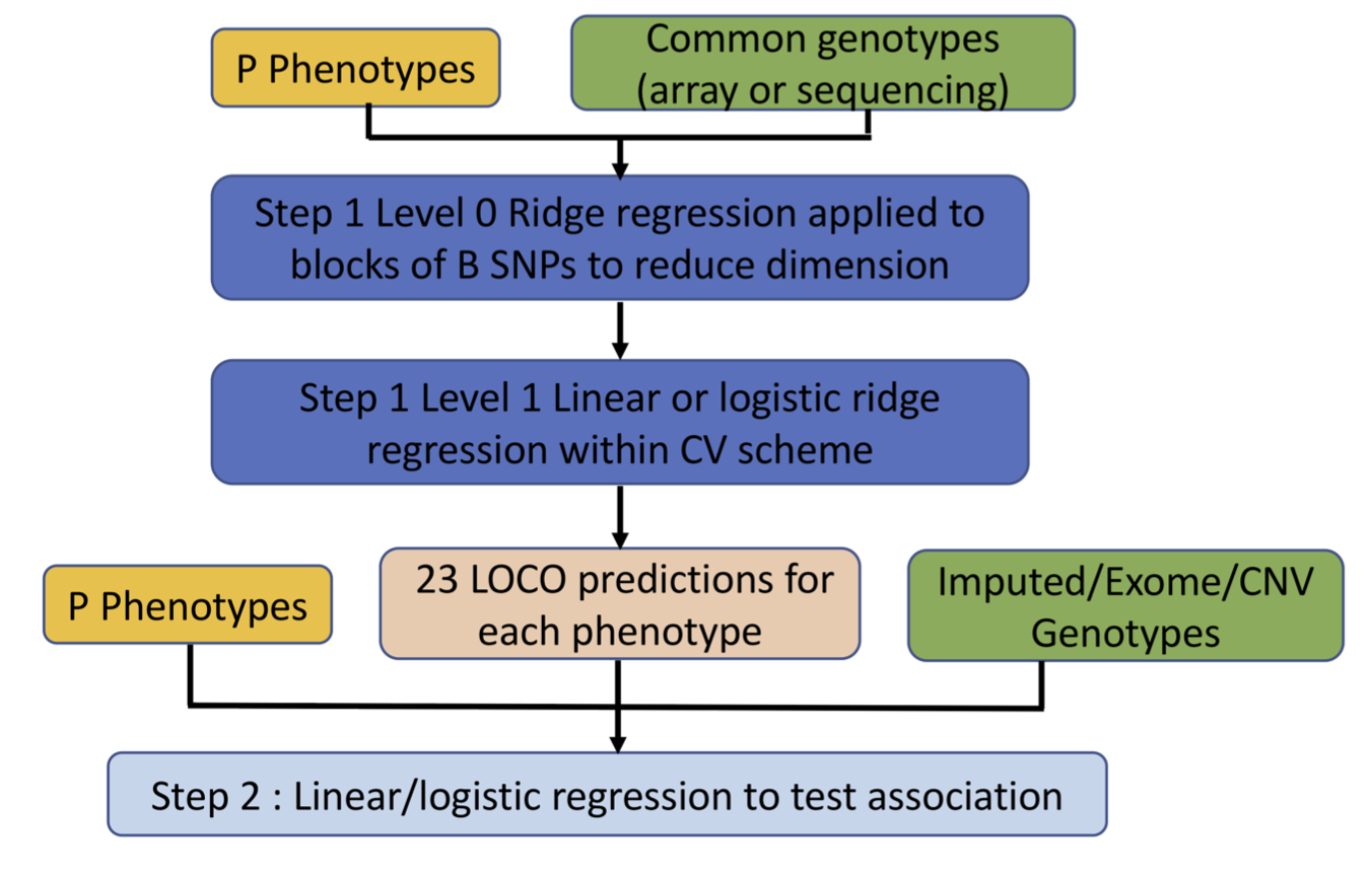
Figure 1. REGENIE Workflow

Mathematical framework of REGENIE

REGENIE conducts whole-genome regression in two computationally efficient steps, making it well-suited for large biobank-scale datasets.

For a quantitative trait, REGENIE begins with the linear mixed model:

\[ y = X\alpha + G \beta + \varepsilon, \tag{1} \]

where $G$ represents the standardised genotype matrix, $\alpha$ denotes the fixed effects of covariates, $\beta$ indicates the effect sizes of genotypes, and $\varepsilon$ is the random noise, characterised by:

\[ \beta \sim N(0, \sigma_g^2 \mathbf{I}), \quad \varepsilon \sim N(0, \sigma_e^2 \mathbf{I}). \]

For a binary trait, the first stage (Level-0) remains the same, while the second stage (Level-1) employs logistic regression via the logit link. In Step 2, logistic regression is again used for association testing.

Foundations of Step 1 in REGENIE

In Step 1 of REGENIE, consider the following notation:

$y \in \mathbb{R}^n$ — phenotype vector (quantitative or binary, after any required transformation)
$X \in \mathbb{R}^{n \times p}$ — fixed-effect covariates (e.g., age, sex, principal components)
$G \in \mathbb{R}^{n \times m}$ — standardised genotype matrix for $m$ variants
$\alpha \in \mathbb{R}^p$ — fixed-effect coefficients
$\beta \in \mathbb{R}^m$ — genome-wide SNP effects
$\varepsilon \in \mathbb{R}^n$ — residual errors

Simplifying the model

The full model is given by:

\[ y = X \alpha + G \beta + \varepsilon. \]

To remove the contribution of the fixed covariates $X$, all variables are projected onto the orthogonal complement of the column space of $X$ using the projection matrix:

\[ P_X = \mathbf{I} - X (X^\top X)^{-1} X^\top. \]

Since $P_X X = 0$, pre-multiplying the model by $P_X$ yields:

\[ \widetilde{y} = \widetilde{G} \beta + \widetilde{\varepsilon}, \tag{2} \]

where:

\[ \widetilde{y} = P_X y, \quad \widetilde{G} = P_X G, \quad \widetilde{\varepsilon} = P_X \varepsilon. \]

Equation (2) is therefore the covariate-adjusted model used in Step 1.
Level-0 Ridge Regression

The matrix $\widetilde{G}$ is partitioned into $B$ non-overlapping blocks:

\[ \widetilde{G} = \big[ \widetilde{G}_1 \; \widetilde{G}_2 \; \cdots \; \widetilde{G}_B \big], \]

where each block $\widetilde{G}_i \in \mathbb{R}^{n \times m_i}$ contains $m_i$ variants.

For each block $\widetilde{G}_i$, ridge regression models are fitted for a set of $J$ penalty parameters $\{\lambda_1, \ldots, \lambda_J\}$:

\[ \widehat{\beta}_{i, \lambda_j} = \arg\min_{\beta \in \mathbb{R}^{m_i}} \left\{ \|\widetilde{y} - \widetilde{G}_i \beta\|_2^2 + \lambda_j \|\beta\|_2^2 \right\}. \]

The fitted predictors for block $i$ and penalty $\lambda_j$ are:

\[ \widehat{y}_{i, \lambda_j} = \widetilde{G}_i \widehat{\beta}_{i, \lambda_j}. \]

This produces $J \times B$ predictors in total:

\[ \widehat{Y}^{(0)} = \big[ \widehat{y}_{1,\lambda_1}, \dots, \widehat{y}_{1,\lambda_J}, \widehat{y}_{2,\lambda_1}, \dots, \widehat{y}_{B,\lambda_J} \big]. \]

Since each block can be processed independently, this stage is highly parallelisable, substantially reducing computational cost.
Level-1 Ridge Regression (LOCO)

In the second stage, the $J \times B$ predictors from Level-0 are combined via ridge regression:

\[ \widehat{\gamma} = \arg\min_{\gamma \in \mathbb{R}^{J B}} \left\{ \|\widetilde{y} - \widehat{Y}^{(0)} \gamma\|_2^2 + \lambda^{(1)} \|\gamma\|_2^2 \right\}. \]

Here, $\lambda^{(1)}$ is selected from a set of shrinkage parameters to minimise the prediction error.

REGENIE employs a Leave-One-Chromosome-Out (LOCO) procedure to avoid proximal contamination:
- For each chromosome $c$, predictors derived from variants on chromosome $c$ are excluded when fitting the Level-1 model.
- The resulting LOCO predictor, $\widehat{y}^{(1)}_{(-c)}$, is used in Step 2 when testing variants on chromosome $c$.
- This generates 22/23 LOCO predictions for a human dataset.

Running GWAS with REGENIE

EXERCISE 11 (Optional): Running REGENIE Interactively (Quantitative Trait)

dir_data="${dir_user}/snake-cma/examples/data"
dir_cma="${dir_user}/snake-cma/examples/cma-tests"

mkdir -p "${dir_cma}"

geno="${dir_data}/HAPMAP3.qc.genotype"
pheno="${dir_data}/continuous_trait.phen"
covars="${dir_data}/HAPMAP3.covars.cov"
output="${dir_cma}/ex11-regenie-qt"

reg="${dir_user}/snake-cma/examples/software/regenie/regenie_v3.2.1.gz_x86_64_Linux"
plink2="${dir_user}/snake-cma/examples/software/plink2/plink2"

echo "Starting..."

# REGENIE Step 1
"${reg}" \
  --step 1 \
  --bed "${geno}" \
  --phenoFile "${pheno}" \
  --covarFile "${covars}" \
  --bsize 1000 \
  --lowmem \
  --lowmem-prefix "${output}_step1_cache" \
  --out "${output}_step1"

# REGENIE Step 2
"${reg}" \
  --step 2 \
  --bed "${geno}" \
  --phenoFile "${pheno}" \
  --covarFile "${covars}" \
  --pred "${output}_step1_pred.list" \
  --bsize 2000 \
  --minMAC 20 \
  --out "${output}_step2"

echo "Done."

EXERCISE 12: Run GWAS with REGENIE for a quantitative trait via a Bash script

Goal: Write and run a small Bash script that runs REGENIE for a quantitative trait. Make sure to change the output variable to a unique name before running.

Show solution

Create the script file:
```
nano ex12.sh
```

Paste the solution below, then save and close:

#!/bin/bash
set -euo pipefail

dir_user="${1:?ERROR: provide repo root as first argument}"
dir_data="${dir_user}/snake-cma/examples/data"
dir_cma="${dir_user}/snake-cma/examples/cma-tests"

mkdir -p "${dir_cma}"

geno="${dir_data}/HAPMAP3.qc.genotype"
pheno="${dir_data}/continuous_trait.phen"
covars="${dir_data}/HAPMAP3.covars.cov"
output="${dir_cma}/ex12-regenie-qt"
reg="${dir_user}/snake-cma/examples/software/regenie/regenie_v3.2.1.gz_x86_64_Linux"

echo "Starting..."

# REGENIE Step 1
"${reg}" \
  --step 1 \
  --bed "${geno}" \
  --phenoFile "${pheno}" \
  --covarFile "${covars}" \
  --bsize 1000 \
  --lowmem \
  --lowmem-prefix "${output}_step1_cache" \
  --out "${output}_step1"

# REGENIE Step 2
"${reg}" \
  --step 2 \
  --bed "${geno}" \
  --phenoFile "${pheno}" \
  --covarFile "${covars}" \
  --pred "${output}_step1_pred.list" \
  --bsize 2000 \
  --minMAC 20 \
  --out "${output}_step2"

echo "Done."

Run the script (pass the repository root you saved earlier as dir_user):
```
bash ex12.sh "${dir_user}"
```

EXERCISE 13 (Optional): Run GWAS with REGENIE for a quantitative trait using an HPC job script on your cluster

Goal: Write and run a small job script for your local HPC cluster that runs REGENIE for a quantitative trait. Make sure to change the output variable to a unique name before running.

Show solution

A solution for Eddie (the University of Edinburgh HPC cluster) will be provided during the in-person training.

EXERCISE 14: Running REGENIE Interactively (Binary Trait)

dir_data="${dir_user}/snake-cma/examples/data"
dir_cma="${dir_user}/snake-cma/examples/cma-tests"

mkdir -p "${dir_cma}"

geno="${dir_data}/HAPMAP3.qc.genotype"
pheno="${dir_data}/binary_trait.phen"
covars="${dir_data}/HAPMAP3.covars.cov"
output="${dir_cma}/ex14-regenie-bt"

reg="${dir_user}/snake-cma/examples/software/regenie/regenie_v3.2.1.gz_x86_64_Linux"
plink2="${dir_user}/snake-cma/examples/software/plink2/plink2"

echo "Starting..."

# REGENIE Step 1
"${reg}" \
  --step 1 \
  --bed "${geno}" \
  --phenoFile "${pheno}" \
  --covarFile "${covars}" \
  --bsize 1000 \
  --lowmem \
  --bt \
  --lowmem-prefix "${output}_step1_cache" \
  --out "${output}_step1"

# REGENIE Step 2
"${reg}" \
  --step 2 \
  --bed "${geno}" \
  --phenoFile "${pheno}" \
  --covarFile "${covars}" \
  --pred "${output}_step1_pred.list" \
  --bsize 2000 \
  --minMAC 20 \
  --bt \
  --firth --approx \
  --out "${output}_step2"

echo "Done."

EXERCISE 15: Run GWAS with REGENIE for a binary trait via a Bash script

Goal: Write and run a small Bash script that runs REGENIE for a binary trait. Make sure to change the output variable to a unique name before running.

Show solution

Create the script file:
```
nano ex15.sh
```

Paste the solution below, then save and close:

#!/bin/bash
set -euo pipefail

dir_user="${1:?ERROR: provide repo root as first argument}"
dir_data="${dir_user}/snake-cma/examples/data"
dir_cma="${dir_user}/snake-cma/examples/cma-tests"

mkdir -p "${dir_cma}"

geno="${dir_data}/HAPMAP3.qc.genotype"
pheno="${dir_data}/binary_trait.phen"
covars="${dir_data}/HAPMAP3.covars.cov"
output="${dir_cma}/ex15-regenie-bt"

reg="${dir_user}/snake-cma/examples/software/regenie/regenie_v3.2.1.gz_x86_64_Linux"

echo "Starting..."

# REGENIE Step 1
"${reg}" \
  --step 1 \
  --bed "${geno}" \
  --phenoFile "${pheno}" \
  --covarFile "${covars}" \
  --bsize 1000 \
  --lowmem \
  --bt \
  --lowmem-prefix "${output}_step1_cache" \
  --out "${output}_step1"

# REGENIE Step 2
"${reg}" \
  --step 2 \
  --bed "${geno}" \
  --phenoFile "${pheno}" \
  --covarFile "${covars}" \
  --pred "${output}_step1_pred.list" \
  --bsize 2000 \
  --minMAC 20 \
  --bt \
  --firth --approx \
  --out "${output}_step2"

echo "Done."

Run the script (pass the repository root you saved earlier as dir_user):
```
bash ex15.sh "${dir_user}"
```

EXERCISE 16 (Optional): Run GWAS with REGENIE for a binary trait using an HPC job script on your cluster

Goal: Write and run a small job script for your local HPC cluster that runs REGENIE for a binary trait. Make sure to change the output variable to a unique name before running.

Show solution

A solution for Eddie (the University of Edinburgh HPC cluster) will be provided during the in-person training.

Introduction to CMA

Corrected Meta-Analysis (CMA) is a divide-and-conquer approach designed for efficient genome-wide association studies on very large datasets. The method splits the data into smaller, more manageable chunks, runs association analyses in parallel using tools such as REGENIE or fastGWA-GLMM, and then combines the results through a novel meta-analysis method that accounts for between-cohort confounders. This workflow reduces computational burden significantly, allows flexible use of high-performance computing resources, and makes large-scale GWAS feasible even with limited per-job memory or runtime constraints.

CMA separates the predictivity stage (estimation of effect sizes) from the discovery stage (identification of loci or generation of p-values). In the predictivity stage, it mitigates the “winner’s curse” effect, providing better-calibrated effect size estimates. In the discovery stage, it achieves equally as good discovery levels as the gold standard GWAS methods such as REGENIE.

CMA workflow schematic

Step	Description
Split	Partition cohort into $M$ sub-cohorts ($M$ is defined by the user)
Analyse	Run GWAS for each sub-cohort in parallel
Combine	Merge and meta-analyse results

\[ \boxed{\quad \text{Data} \quad} \xrightarrow{\mathbf{split}} \boxed{\quad \text{Sub-cohort 1},\ \text{Sub-cohort 2},\ \ldots \quad} \xrightarrow{\mathbf{GWAS\ (in\ parallel)}} \boxed{\quad \widehat{\beta}_1,\ \widehat{\beta}_2,\ \ldots \quad} \xrightarrow{\mathbf{corrected\ meta\text{-}analysis}} \boxed{\quad \widehat{\beta}_{\text{final}} \quad} \]

Quantifying Relationships Between Sub-cohorts in CMA

When combining results from multiple sub-cohorts into a single estimate, it is important to account for the degree of overlap in information between sub-cohorts, which can arise from the presence of related individuals distributed across different sub-cohorts.. Overlap affects how similar the separate results are to one another, and failing to adjust for it can bias the combined result.

CMA incorporates this overlap adjustment through the following relationship:

\[ \mathrm{Corr}(\widehat{\beta}_i, \widehat{\beta}_j) = \gamma_{12} \, \mathrm{Corr}(z_i, z_j), \]

where:

$z_i$ and $z_j$ are the z-scores from the GWAS results of cohorts $i$ and $j$, respectively,
$\gamma_{12}$ is defined as: \[ \gamma_{12} = \begin{cases} -1, & \text{if } \widehat{\beta}_i \cdot \widehat{\beta}_j < 0, \\ \;\;1, & \text{otherwise}. \end{cases} \]

CMA Predictivity

By modelling and adjusting for the correlation structure arising from cohort overlap, CMA produces effect size estimates that are better calibrated and less biased compared to standard GWAS. This yields improved predictive performance when the resulting polygenic scores are applied to independent datasets.

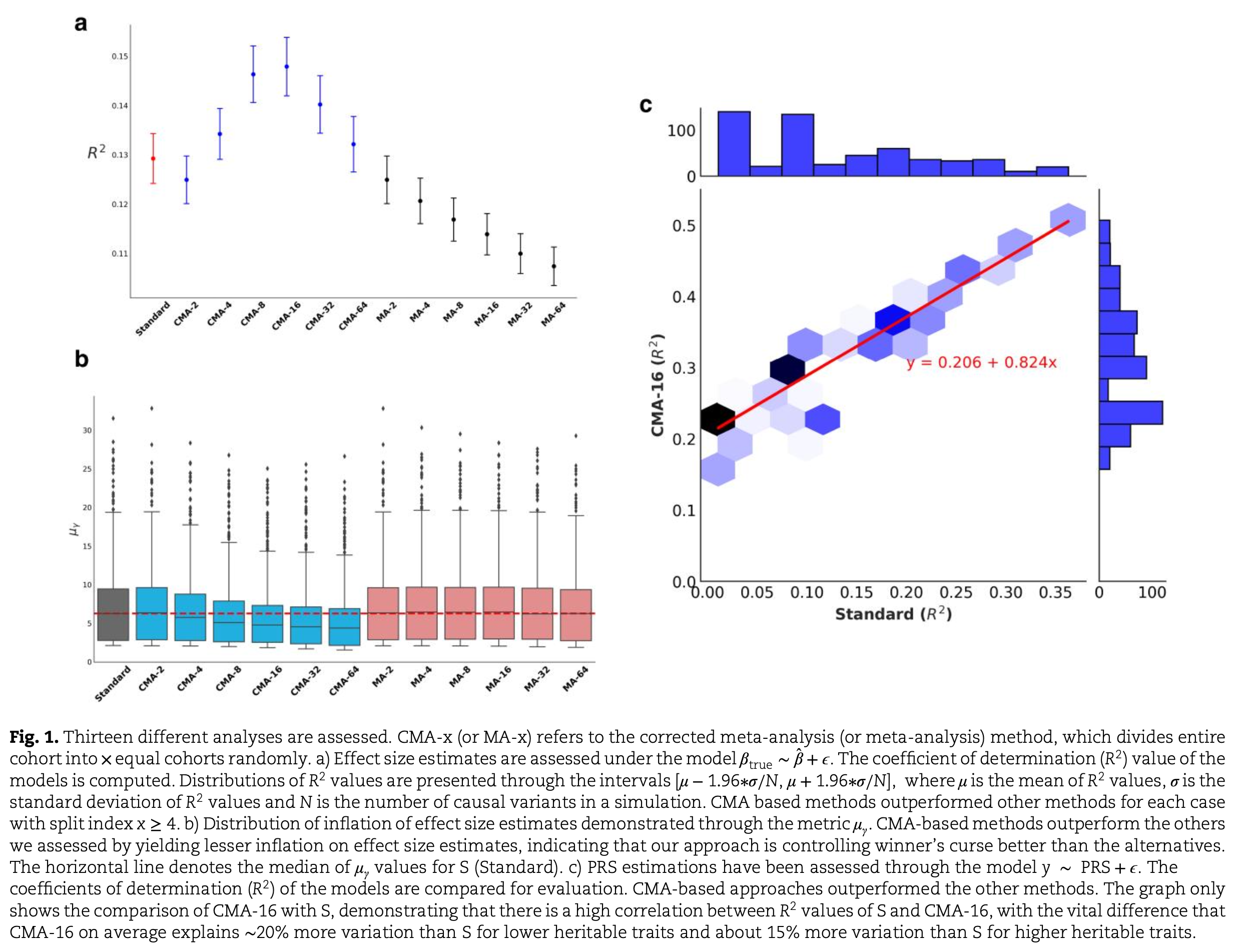
CMA Discovery

CMA achieves lower false discovery rates than standard GWAS methods, although this comes at the expense of some statistical power. For those prioritising higher power, CMA includes an inflation-based summary statistics option that enables discovery levels comparable to standard GWAS approaches. This is made possible by CMA’s decoupled framework for prediction and discovery.

We applied CMA to 12 traits from the UK Biobank using the inflation mode. CMA maintained discovery power equivalent to that of REGENIE in terms of genome-wide significant loci.

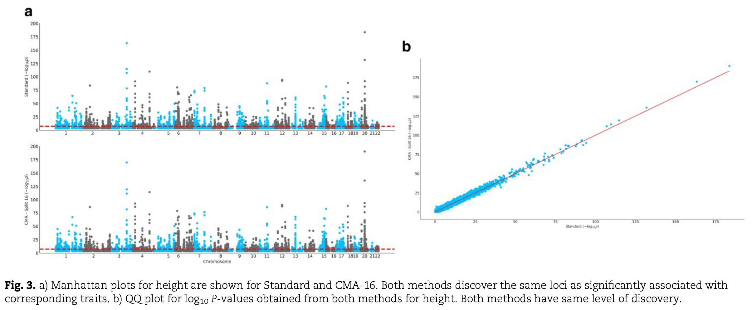
A Manhattan plot is a scatter plot commonly used in GWAS to display –log₁₀ p-values of genetic variants across the genome, with chromosomes arranged sequentially along the x-axis. It is used to visualise and identify genomic regions with strong association signals. A Q–Q plot compares the observed distribution of test statistics (such as p-values) with the expected distribution under the null hypothesis. In the figure above, it is used to compare the distributions of GWAS summary results obtained from CMA and REGENIE.

Computational Benchmark of CMA

Extensive benchmarking demonstrates that CMA offers substantial computational advantages over both REGENIE and fastGWA-GLMM. It enables GWAS to be performed on large-scale datasets using only moderate computing resources if required; for example, CMA can run efficiently on datasets containing 5 million individuals.

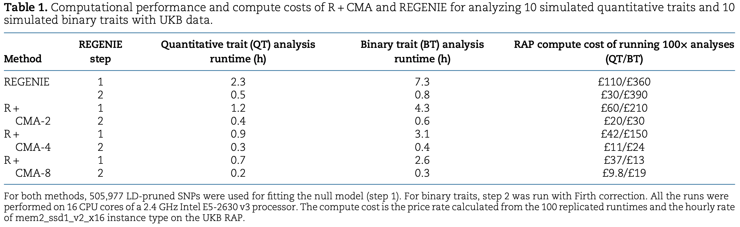
R + CMA (or RCMA in short) indicates that CMA is used in conjunction with REGENIE to perform GWAS on sub-cohorts.

CMA as a Multi-Purpose Tool

CMA is a versatile framework for large-scale genetic association studies, offering both GWAS execution and meta-analysis within the same framework. For GWAS, CMA supports running REGENIE (RCMA) and fastGWA-GLMM (FCMA) directly with a split of 1 (i.e. $M=1$), producing results identical to running each method natively. When a split index greater than 1 is specified, CMA automatically partitions the dataset, runs GWAS on each subset in parallel, and then combines the results, enabling efficient analysis of datasets without loosing any statistical discovery. In addition, CMA implements a unique meta-analysis method that corrects for related individuals across sub-cohorts, currently the only approach offering this capability.

Key capabilities of CMA:

GWAS modes:
- REGENIE (RCMA with split = 1)
- fastGWA-GLMM (FCMA with split = 1)
- RCMA/FCMA with split > 1
Meta-analysis mode (Not covered in this tutorial):
- CMA that accounts for relatedness between sub-cohorts

Running GWAS with CMA

EXERCISE 17: Run GWAS with CMA via a Bash script

Goal: Write and run a small job script for CMA, using either R + CMA (RCMA) or F + CMA (FCMA), which splits the cohort into 2 sub-cohorts for a binary trait.

Show solution

The downloaded repository already includes the necessary Bash scripts, with RCMA and FCMA options providing the solution to this exercise. The script rcma.qt.sh can also be tested on a quantitative trait, although this run takes considerably longer to complete.

# Option A: R+CMA — REGENIE (Quantitative)
bash ./snake-cma/examples/rcma.qt.sh

# Option B: R+CMA — REGENIE (Binary)
bash ./snake-cma/examples/rcma.bt.sh

# Option C: F+CMA — fastGWA-GLMM (Binary)
bash ./snake-cma/examples/fcma.bt.sh

EXERCISE 18: Run REGENIE with CMA

Goal: Run R + CMA (RCMA) with a single split (i.e. $M=1$) to execute REGENIE under the CMA framework.

Show solution

dir_data=${dir_user}/snake-cma/examples/data
dir_cma=${dir_user}/snake-cma/examples/cma-tests

mkdir -p ${dir_cma}

geno=${dir_data}/HAPMAP3.qc.genotype
pheno=${dir_data}/binary_trait.phen
covars=${dir_data}/HAPMAP3.covars.cov
output=${dir_cma}/ex18-rcma-bt-split1

reg=${dir_user}/snake-cma/examples/software/regenie/regenie_v3.2.1.gz_x86_64_Linux
plink2=${dir_user}/snake-cma/examples/software/plink2/plink2
cma=${dir_user}/snake-cma/src/snake_cma.py

echo Starting..
python ${cma} \
    --bed ${geno} \
    --bt \
    --split 1 \
    --out ${output} \
    --phenoFile ${pheno} \
    --covarFile ${covars} \
    --regenie ${reg} \
    --plink ${plink2}

echo Done..

EXERCISE 19: Run fastGWA-GLMM with CMA

Goal: Run F + CMA (FCMA) with a single split (i.e. $M=1$) to execute fastGWA-GLMM under the CMA framework.

Show solution

dir_data=${dir_user}/snake-cma/examples/data
dir_cma=${dir_user}/snake-cma/examples/cma-tests

mkdir -p ${dir_cma}

geno=${dir_data}/HAPMAP3.qc.genotype
pheno=${dir_data}/binary_trait.phen
covars=${dir_data}/HAPMAP3.covars.qcovar
output=${dir_cma}/ex19-fcma-bt-split1

reg=${dir_user}/snake-cma/examples/software/regenie/regenie_v3.2.1.gz_x86_64_Linux
plink2=${dir_user}/snake-cma/examples/software/plink2/plink2
cma=${dir_user}/snake-cma/src/snake_cma.py

echo Starting..

# Build sparse GRM only if it doesn't exist
if [ ! -f "${grm}.grm.sp" ]; then
  ${gcta} --bfile ${geno} \
      --make-grm \
      --sparse-cutoff 0.05 \
      --out ${grm}
fi

python ${cma} \
    --bt \
    --bed ${geno} \
    --sp-grm ${grm} \
    --split 1 \
    --out ${output} \
    --phenoFile ${pheno} \
    --covarFile ${covars} \
    --gcta ${gcta} \
    --plink ${plink2} \
    --joint_covar

echo Done..

(Optional) Running Meta-Analysis with CMA

EXERCISE 20: Run Meta-Analysis with CMA via a Bash script

Goal: Combine GWAS results from fastGWA-GLMM or REGENIE using the CMA meta-analysis approach.

Show solution

# Option D: CMA Meta-analysis — Quantitative
bash ./snake-cma/examples/cma.qt.sh

# Option E: CMA Meta-analysis — Binary
bash ./snake-cma/examples/cma.bt.sh

💬 Questions / Comments / Feedback

Thank you for joining this training session on Scalable Methods for Large-Scale Genetic Association Studies.

In this session, we covered three major GWAS tools REGENIE, fastGWA/fastGWA-GLMM, and CMA, explored their core concepts, and showed how to run them through hands-on examples with sample datasets.

This concludes our tutorial. Now is the time for any remaining questions or comments before we wrap up.

If you have questions in the future or need additional clarification, please don’t hesitate to reach out:

İsmail Özkaraca: ozkaraca AT duck DOT com

References

[1] (REGENIE) Mbatchou, J., Barnard, L., Backman, J. et al. Computationally efficient whole-genome regression for quantitative and binary traits. Nat Genet 53, 1097–1103 (2021). https://doi.org/10.1038/s41588-021-00870-7

[2] (fastGWA) Jiang, L., Zheng, Z., Qi, T. et al. A resource-efficient tool for mixed model association analysis of large-scale data. Nat Genet 51, 1749–1755 (2019). https://doi.org/10.1038/s41588-019-0530-8

[3] (fastGWA-GLMM) Jiang, L., Zheng, Z., Fang, H. et al. A generalized linear mixed model association tool for biobank-scale data. Nat Genet 53, 1616–1621 (2021). https://doi.org/10.1038/s41588-021-00954-4

[4] (GCTA) Yang, Jian, et al. “GCTA: a tool for genome-wide complex trait analysis.” The American Journal of Human Genetics 88.1 (2011): 76-82. https://doi.org/10.1016/j.ajhg.2010.11.011

[5] (CMA) Mustafa İsmail Özkaraca, Mulya Agung, Pau Navarro, Albert Tenesa, Divide and conquer approach for genome-wide association studies, Genetics, Volume 229, Issue 4, April 2025, iyaf019, https://doi.org/10.1093/genetics/iyaf019

[6] Listgarten, J., Lippert, C., Kadie, C. et al. Improved linear mixed models for genome-wide association studies. Nat Methods 9, 525–526 (2012). https://doi.org/10.1038/nmeth.2037

Step	Description
Split	Partition cohort into \(M\) sub-cohorts (\(M\) is defined by the user)
Analyse	Run GWAS for each sub-cohort in parallel
Combine	Merge and meta-analyse results

Training-3

Contents

Brief Overview of GWAS

Simple Linear Regression in GWAS:

Confounders in GWAS:

Linear Mixed Models (LMMs) in GWAS

Solving LMMs in GWAS

Hypothesis Testing in GWAS (LMMs)

Evidence of Association in GWAS LMMs

GWAS Requires Large Sample Sizes

Installing the Software and Dataset

Introduction to fastGWA and fastGWA-GLMM

Linear Mixed Model for Quantitative Traits

Generalized Linear Mixed Model for Binary Traits

Computational Note

Running GWAS with fastGWA and fastGWA-GLMM

EXERCISE 1: Running fastGWA Interactively (Quantitative Trait)

EXERCISE 2: Perform GWAS with fastGWA interactively using both –qcovar and –covar options

EXERCISE 3: Run GWAS with fastGWA via a Bash script

EXERCISE 4 (Optional): Run GWAS with fastGWA using an HPC job script on your cluster

EXERCISE 5: Running fastGWA-GLMM Interactively (Binary Trait)

EXERCISE 6: Run GWAS with fastGWA-GLMM via a Bash script

EXERCISE 7: Run GWAS with fastGWA-GLMM via a Bash script using only quantitative covariates

EXERCISE 8 (Optional): Run GWAS with fastGWA using an HPC job script on your cluster

EXERCISE 9: Run GWAS with Multiple Phenotypes using fastGWA or fastGWA-GLMM

EXERCISE 10 (Optional): Split GRM Calculation

Introduction to REGENIE

Mathematical framework of REGENIE

Foundations of Step 1 in REGENIE

Running GWAS with REGENIE

EXERCISE 11 (Optional): Running REGENIE Interactively (Quantitative Trait)

EXERCISE 12: Run GWAS with REGENIE for a quantitative trait via a Bash script

EXERCISE 13 (Optional): Run GWAS with REGENIE for a quantitative trait using an HPC job script on your cluster

EXERCISE 14: Running REGENIE Interactively (Binary Trait)

EXERCISE 15: Run GWAS with REGENIE for a binary trait via a Bash script

EXERCISE 16 (Optional): Run GWAS with REGENIE for a binary trait using an HPC job script on your cluster

Introduction to CMA

CMA workflow schematic

Quantifying Relationships Between Sub-cohorts in CMA

CMA Predictivity

CMA Discovery

Computational Benchmark of CMA

CMA as a Multi-Purpose Tool

Running GWAS with CMA

EXERCISE 17: Run GWAS with CMA via a Bash script

EXERCISE 18: Run REGENIE with CMA

EXERCISE 19: Run fastGWA-GLMM with CMA

(Optional) Running Meta-Analysis with CMA

EXERCISE 20: Run Meta-Analysis with CMA via a Bash script

💬 Questions / Comments / Feedback

References